Though QGD predicts the existence of structures which exerts such gravitational pull that photons cannot escape. But contrary to the classical black holes predicted by relativity, the black holes predicted by quantum-geometry dynamics are not singularities. The QGD exclusion principle which states that a preon(-) cannot be occupied by more than one preon(+) implies that quantum-geometrical space imposes a limit to the density any structure can have. The density of black holes is also limited by the fact that preons(+), being strictly kinetic, they must have enough space to keep in motion. It follows that black must have very large yet finite densities.

Angle between the Rotation Axis and the Magnetic Axis

The effect of the helical motions of the electrons in direction of the rotation of a body adds up so that, at a large scale, the body behaves as a single large electron which though helical trajectory around the body interacts with the neighbouring preonic region to generated a magnetic field.

Since the magnetic field is the result of the polarization of free along the loops of the helical trajectory, and since the inclination of these loops increase with the rotation speed, so does the angle between these loops and the axis of rotation increases. It follows that the angle between the axis of rotation and the magnetic axis for bodies of given material composition is proportional to the speed of rotation about its axis and its diameter.

This angle between the axis of rotation and the magnetic axis is small for slowly rotating bodies but can never be so small that the axes coincide. From the above, it also follows that a faster rotation not only implies a larger the angle between the rotation axis and the magnetic axis is, but also a flattening of the magnetic field and an increase in its intensity.

The Inner Structure of Black Holes

To understand the structure of a black hole we will look at what happens to a photon when it is captured by it the gravitational pull.

The model for light refraction that we introduced in earlier articles can be applied directly to photon moving through a black hole. Since we assume that the black hole is extremely massive, its trajectory will bring it towards the center of the black hole.

When moving along the magnetic axis of the black hole, the component of the pairs of the photon are pulled away from each other, splitting the photon into free which may or not recombine into neutrinos. This works as follow:

As we have seen earlier in this book, the force binding the of a pairs is gravitational. The QGD gravitational interaction between particles at the fundamental scale is , and since and are , and since , the binding force between two of a pair is equal to .

For a photon moving along the magnetic axis, we have and where and are the component of a pair of a photon.

The regions and , on each side of the black hole axis are equally massive regions. If we call and the regions each side of when the photon’s trajectory is aligned with the black hole axis then and . Similarly, if we call and the region on the each side then and . So the force pulling the of pairs being greater than the force that binds them, the pairs are split into single .

How do we that the gravitational forces within a black hole are sufficiently strong to cause the photons to be broken down into ? If the gravitational forces within the black hole were not enough to breakdown the photons, then photons moving along a black hole axis would escape into space making the black hole visible. Since black holes do not emit light, then the gravitational interactions must be strong enough to break photons down into and neutrinos.

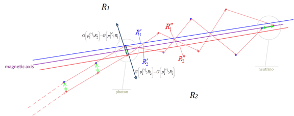
The image above shows how a simple two photon is split into two free which because of the the electro-gravitational interactions move back toward the magnetic axis. But, because the quantum-geometrical space occupied by the black holes is densely populated by particles which affect randomly the trajectories of the single , our two arrive at the magnetic axis of the black hole at different positions. And if they are in close enough proximity, the single will combine to form a neutrino which structure, not being made of pairs, remains structurally unaffected by the intense gravitational interactions within the black hole.

Once the trajectories of the or the neutrino coincides with the magnetic axis of the black hole, the or neutrinos will move through the center of the black hole and will exit it. and neutrinos can escape the gravitation of the black hole because gravitational interactions, though it affects the directions of , doesn’t change their momentums which, as we have seen in earlier articles is fundamental and intrinsic (the momentum of a is where is momentum vector of a ).

It follows, that all matter that falls into a black hole will be similarly disintegrated into and neutrinos, which will exit the black hole. The black hole will thus radiate and neutrinos, in jets at both poles of their magnetic axis of rotation. Since and neutrinos interact too weakly with instruments to be detected by our instruments, they are invisible to them. In order to see the -neutrinos jets from a black hole, instruments may need detectors larger than our solar system. However, the jets can be observed indirectly when they interact with large amount of matter when the polarized and neutrinos they contain impart it with their intrinsic momentum. It is worth noting that polarized preons and neutrinos jets, as described by QGD, would contribute to the observed dark energy effect.

Based on QGD’s model of the black hole, we can predict that the /neutrino jets will form an extremely intense polarized field along the magnetic axis creating the equivalent of a repulsive electromagnetic effect at both poles. The polarized preonic field would repulse all matter on their path, which may explain the shape of galaxies.

From what we have discussed in the preceding section, we can define a black hole as an object which mass is such that it can breakdown all matter, including photons, into .

The QGD model of the physics of black hole has another important implication. The and neutrinos resulting from the breakdown of a particle or structure are indistinguishable from the or neutrinos resulting from the breakdown of any other particle or structure. This means, if QGD is correct, that all information about the original particle or structure is lost forever. That said, since this consistent from QGD’s axioms set and since, unlike quantum mechanics, QGD does not require that information be preserved, the loss of information it predicts does not lead to a paradox ( see this article for an excellent introduction to subject).

Cosmological Consequences

The mechanism of emission of and neutrinos will be continue until the black hole has been completely evaporated; which it will after it has absorbed all matter in its vicinity. By this mechanism, which had formed particles and structures are disintegrated into free and neutrinos which are then returned to the universe.

In later phases, the free and neutrinos will form new particles and structures, eventually leading to the formation cosmic structures and black holes. And later, due to gravitational interactions, these cosmic structures will ultimately be absorbed by black holes, which break down matter into and neutrinos, repeating the cycle indefinitely.

For a more complete discussion on the subject, see relevant sections in Introduction to Quantum-Geometry Dynamics.

Note: to fully appreciate and understand the following discussion, I highly recommend reading the article titled
A Remarkably Simple Proof of the Discreteness of Space . Also, for an explanation of the fundamental mechanism which governs momentum transfer, you may read the article Baseball Physics as Explained by Quantum-Geometry Dynamics.

Everyone is familiar with Newton’s Cradle, a simple mechanism which is thought to demonstrate the law of conservation of momentum. Paradoxically, the physics of Newton struggles to describe and explain the behaviour of this simple system of steel balls. In fact, even the full power of continuous mathematics can only provide an approximation of the behaviour of such a system and even that must be at the cost of undesirable and awkward complications.

The reader may ask why, today, anyone should bother trying to explain such a trivial device when there are so many exciting phenomena to which quantum-geometry dynamics can be applied. Let me ask this question: How can Newton’s cradle be a device demonstrating Newton’s laws of motion when Newton’s laws of motion cannot explain its behaviour? Also, since quantum-geometry dynamics claims to explain the dynamics of motion at all scales (and do so in as a simple and straightforward way), applying it successfully to Newton’s cradle should be easy. Not to mention, an excellent opportunity to test its validity. It also doesn’t hurt that building any version of Newton’s cradle is considerably less expensive than, let’s say, a particle accelerator.

The first thing we must do is formulate the problem in QGD terms. Given a Newton’s cradle system having steel balls, when lifting then dropping subset consisting of numbers of balls, the impact with set number of balls will in motion. The problem will be to predict and explain which balls will be set in motion from the impact as well as determine their momentum and speed.

We have explained earlier articles that QGD defines the momentum of an object as and the its speed as where is its mass in preons(+). Thus momentum and speed are intrinsic properties independent of the frame of reference.

We also know that the preons(-), the elementary particle that dimensionalizes space to form quantum-geometrical space, generating an opposing force to changes in momentum so that it only allows changes in momentum when where .

Conservation of momentum (which is a consequence of the conservation of the fundamental momentum of preons(+)) is such that where and are respectively the momentum of a group of balls pulled and released together and the momentum of the group of balls set in motion after impact.

Also since where , we have or and since then . That is, the momentum transferred must be an integer multiple of the mass of a ball. This all we need to explain and predict the behaviour of a Newton’s cradle system from initial conditions are known. Let’s examine now a few examples showing how the above applies.

In the example shown in the figure on the left, which leave balls on the right. Now, we know that the momentum can only be transferred in integer multiples of , and since the three balls carry an integer multiple of (equivalent to an integer number of balls), if it were to be transferred to the remaining two balls, the resulting change of momentum for each ball would be a non-integer. Non-integer changes in momentum are forbidden by structure of quantum-geometrical space.

So the total momentum that can be transferred to the two red balls is , each, but since the total momentum of the blue balls is that leaves us with . Since the remaining momentum cannot be transferred, it will be kept by the blue balls. But here again, it cannot be divided between the three blue balls, which would imply them having momentums that are non-integer multiples of . The remaining momentum will be kept by one of the balls, which evidently is the blue ball on the right. The result will be as shown in the figure on the left.

The example above shows a configuration where , leaving one ball. Applying what we’ve learned above, we see that four is divisible by one. Then the entire momentum of the blue balls can be transferred to the red ball. Using QGD definitions we gave at the beginning of this article, we find that the speed of red ball is four times that of the speed of the group of blue balls.

Now, let’s make thing a little more complicated by using a cradle where the balls are of different mass.

The cradle above is made using balls having different mass. With the large balls being exactly twice as massive as the smaller balls. In the figure above, will not represent the number of balls pulled, since we have balls of two different masses, but the equivalent number of small balls. So here . Using the same logic as above, the momentum of the blue balls will be transferred in its entirety to one ball.

Now, some readers may ask why can’t the momentum of the blue balls be transferred to three red balls instead since such change in momentums are integer multiples of (here is the mass of a small ball). The answer is that if a ball can transfer its momentum it will. Transfer of momentum is compulsory if possible and in the example above, the successive balls from impact can transfer the momentum and so they do. The last red ball has no other ball to transfer the momentum to, so it must carry it. And its speed will be three times that of the group of blue balls before impact.

Allow me one last example using the cradle above.

In the above figure , but the momentum cannot be transferred completely to the red balls. can be transferred to the six red balls on the left, leaving us with . But is required to move the large red ball and fractional changes in momentum being forbidden, the remaining momentum cannot be transferred to it. As a result, it must be kept by one of the blue balls. The blue ball that will carry the remaining with be the one on the left. And since it cannot move towards the right, to conserve momentum, it will have to be reflected back to the left (see figure below).

I leave it to the reader to figure out what in this last example when the blue ball on the left and the group of red balls on the right swing back to impact the remain balls. But that shouldn’t be difficult using the notions presented in this article.

Finally, as discussed in the article titled A Remarkably Simple Proof of the Discreteness of Space , the transfer of momentum produces a nearly instant acceleration of the balls that are set in motion from the impact. Such an acceleration, if space were continuous and speed and momentum described classically, would require a nearly infinite force. The balls that are set in motion do not accelerate from rest to the speed after impact by going through all the intermediary speeds between them. The balls, QGD predicts, will move instantly go from rest to the speed that corresponds to the momentum transferred to them. And only after impact will they slow down from the effect of gravity. Testing that prediction should be easy enough using a high speed camera.

What we have shown here is that Newton’s cradle can be used to demonstrate at our scale QGD’s concepts of speed, momentum and conservation of momentum which we have used so far to describe the motion of particles and structures at the fundamental scale. It follows that the laws of motion at all scales are consequences of the fundamental scale interactions. As in the previous article, A Remarkably Simple Proof of the Discreteness of Space, we have shown that physics at our scale is the observable consequences of physics at the fundamental scale.

Click here to see a well-made slow motion video of Newton’s cradle in action. Also, readers may be interested in reading Rocking Newton’s Cradle by S. Hutzler, G. Delaney, D. Weaire and F. McLeod) as an example of how complicated it can be to describe even this simple system using classical physics.

A postulate of quantum-geometry dynamics is that space is fundamentally discrete (quantum-geometrical, to be precise). Of course, proving this using our present technology may appear to be beyond difficult especially if, as QGD suggests, the discreteness of space exists at a scale that is orders of magnitude smaller than the Planck scale. The task of proving that space is made of preons(-) may even be impossible because, if as discussed in On Measuring the Immeasurable, fundamental reality lies beyond the limit of the observable. That said, in the same article I explain that though preons(-), which according to QGD is the discrete and fundamental unit of space, and preons(+), its predicted fundamental unit of matter, must be unobservable, their existence implies consequences and effects that must be observable at larger scales.

According to QGD, the momentum of a particle or structure is given by where is the magnitude of the momentum vector of a particle or a structure , the momentum vectors of the component preons(+) of and its mass measured in preons(+). The speed of particle is defined as . We saw that when a structure absorbs a photon of mass , then its new momentum is given by . We also saw that when is subjected to gravitational interaction, , the change in momentum is equal to so that . This is explained in more details in earlier articles. Now, let us see how QGD’s equations can be applied to explain and predict reality at our scale. To illustrate this, we will apply the QGD’s equations to baseball.

Let be a baseball and a baseball bat and let’s look at what happens when the ball, traveling towards the bat at speed is hit by a baseball ball, itself going at speed . Using the definitions above, we know that the momentums of and are respectively given by and and their speed by and . We also know that saw that, if space is quantum-geometrical, any change in momentum of an object must an exact multiple of it mass. That is : . As a consequence, unless the mass of the bat is an exact multiple of the mass of the ball, it cannot transfer all of its momentum to it. Then and , where the brackets represent the floor function. Now what happens to the momentum that is not transferred to the ball? It is conserved the bat in the form of momentum, with part of dissipated by friction and distortion.

Now, since and since , the ball cannot transfer momentum to the bat. The ball retains the momentum it had before the impact (with direction reversed) so that the total momentum of the ball immediately after impact is given by and its speed .

This example shows how the equations used to describe the effect of optical reflection introduced in an earlier article are directly applicable at our scale.

Conservation of momentum is described somewhat accurately by dominant physics theories, but different scales use different sets of equations and even at our scale; the explanations are based on principles which, themselves are not really explained (see the Wikipedia article on Momentum). The problem is that the explanation of conservation of momentum provided by accepted physics theories contains a huge fallacy; one that, though it doesn’t affect its practical usefulness, results in one important oversight. Accepted physics theories can’t describe the acceleration after impact of a baseball, or the acceleration after impact of a billiard ball or that of the steel balls in Newton’s Cradle.

The classical equation for acceleration is given by that equation , which relate force to mass and acceleration. Using this, how exactly does one determine the acceleration of ball after impact with a bat? To do so within the framework of classical physics, we would need to know ,the speed of the ball before impact, and , the speed of the ball after impact, and the time interval over acceleration occurred. From these we can calculate given by . Measuring and is relatively easy. The difficulty is in measuring the time interval ? Is it a thousandth of a second, a millionth of a second?

No one really knows, but we can safely assume that the speed of the ball, as soon as it is no longer in physical contact with the bat, is equal to. So all we really need to know how much time elapses between the moment the ball is in contact with the ball and the moment when it is no longer in contact. Now, that can vary depending on whether the ball is hit head on or at an angle. For the purpose of simplification, let’s assume that the baseball is hit at an angle so that the time of contact is the shortest possible. So how much time elapsed between the “in contact” and “not in contact” states? No existing apparatus can measure this interval for rigid objects, but let’s put the question in equivalent terms of distance and ask: Over what distance does the acceleration occur? The shorter the distance, the shorter the time interval and, using the classical definition of acceleration, the greater the acceleration must be.

Now, if space is continuous, the distance that separate the “in contact” to the “not in contact” states is infinitely small. That is, as small as the distance may be, we can find an intermediate point between the ball and the bat where the bat is not in contact. And if the distance over which the acceleration occurs is infinitesimal, then the is also infinitesimal, that is, so that . And, using Newton’s second law of motion, , since , then . That is, if space is continuous, an infinite amount of force would be necessary to accelerate a baseball in the opposite direction from the point of impact.

Now, some will argue that the time interval of acceleration depends on the rigidity of the materials of the ball and the bat, and since no materials are absolutely rigid, the baseball and bat will remain in contact over a non-infinitesimal distance so that is not infinitesimal and the required force, not infinite. Even if we allow a longer time of contact, the acceleration of the ball only continues for as long as it remains in contact with the bat. The ball stops accelerating as soon as contact is broken. Then, that last bit of acceleration in the transition between the “in contact” and “not in contact” states, must has a definite value, and however small that definite value is, if space is continuous, the distance between those states must infinitesimal and the force required for that last bit of acceleration must be infinite. We know of course that the force is not infinite and that the infinity here is a consequence of the assumption that space is continuous.

Since the distance between the states of “in contact” and “not in contact” cannot be infinitesimal, it follows that space cannot be continuous. And if space is not continuous, then it must be quantum-geometrical. Also, the discreteness of space implies the discreteness of matter. Hence the observation of the conservation of momentum in baseball supports the existence of both preons(-) and preons(+).